Extreme value theory II

In a previous entry we introduced the basics of Extreme Value Theory (EVT), such as the degeneracy of the maxima distribution, the extremal types theorem, as well as the Gumbel, Frechet, Weibull and GEV distributions. In this entry we will see a few examples of random variables and their respective maxima distribution, both theoretical and by performing simulations.

If you like my content, consider following my linkedin page to stay updated.

A few different distributions

Example 1: Consider an i.id. sequence $X_i$ with exponential distribution of parameter $\lambda=1$. Then its CDF is given by $F(x) = 1 - \exp(x)$ for $x > 0$, and let $M_n = \max\{X_1,\dots,X_n \}$. If we take $a_n = 1$ and $b_n = \log n$ we can see that

The first equality follows from the argument in the previous entry and the limit is just the definition of the exponential function. This implies that the maxima of our random variables follows a Gumbel distribution.

Example 2: In this post it is given a sufficient condition to ensure that $M_n$ has Gumbel extremal type (the condition can be found in H.A. David & H.N. Nagaraja (2003), “Order Statistics” (3d edition)). We reproduce here the condition and its applications:

Suppose that the CDF $F$ and density $f$ of $X_i$ are such that

Then $M_n$ has Gumbel extremal type. It also gives a way to compute the sequences $a_n$ and $b_n$: in fact, one can take $a_n = (nf(b_n))^{-1}$ and $b_n =F^{-1}(1-\frac{1}{n})$

Suppose that $X_i$ is an i.i.d. sequence with common distribution $\mathcal{N}(0,1)$. We apply the previous result to the standard normal sequence, where $F(x)=\Phi(x)=\frac{1}{\sqrt{2\pi}}\int_{-\infty}^x e^{-t^2/2}dt$, $f(x)= \phi(x) = \frac{1}{\sqrt{2\pi}} e^{-x^2/2}$ and $F^{-1}(1)=\infty$. Note that using the quotient rule we obtain that the expression in the parenthesis is equivalent to

The first part of the product can be calculated explicitly:

The second part of the product is a bit more delicate: the term $\frac{(1-\Phi(x))}{\phi(x)}$ is known as the Mills ratio of the standard normal distribution. As stated in the article, we have that following asymptotic: $\frac{(1-\Phi(x))}{\phi(x)}\sim \frac{1}{x}$ as $x\to\infty$ (a proof follows immediately from the bounds found in this post). This implies that the limit $L$ is indeed equal to zero, and consequently, $M_n$ has extremal type Gumbel. In this case there is no explicit form for $b_n$, so we will not bother to compute it.

Similarly, if $X\sim\exp(\lambda)$, we have that $F(x)=1-e^{-\lambda x}$, $f(x)=\lambda e^{-\lambda x}$ and $F^{-1}(1)=\infty$. The first part of the product is

while the second part is

hence we have $\frac{d}{dx}\frac{1-F(x)}{f(x)}\equiv0$. As a consequence, $M_n$ has Gumbel extremal type. Additionally, the sequences $a_n$ and $b_n$ can be taken as $b_n = 1 - e^{-\lambda(1-\frac{1}{n})}$ and $b_n = (n\lambda)^{-1}\exp({\lambda(1 - e^{-\lambda(1-\frac{1}{n})})})$.

The same method proves that the extremal type of a Gamma distribution is Gumbel as well.

Example 3: Consider an i.i.d. sequence $X_n$ with uniform distribution $U(0,1)$. Then $F(x) = x$ and $f(x) = 1$ for $[0,1]$. Take $z < 0$ and $n> -z$, and the sequences $a_n = 1/n$ and $b_n = 1$. Then

proving that $M_n$ has Weibull extremal type.

Simulations

In this section we perform some simulations several random variables and see what the distribution of their maxima looks like. The approach we follow is based on obtaining $nk$ samples and group them in $n$ groups of $k$ observations. We compute the maximum for each group and construct the corresponding histogram.

Example 4: consider an i.i.d. sequence $X_i\sim\mathcal{N}(0,1)$, and take $k=50$ and $n=2000$. We generate $100000$ observations of our random variable and group them in $2000$ groups of $50$ samples.

import numpy as np
import matplotlib.pyplot as plt
from scipy.stats import expon

n = 2000
k = 50
obs = n*k

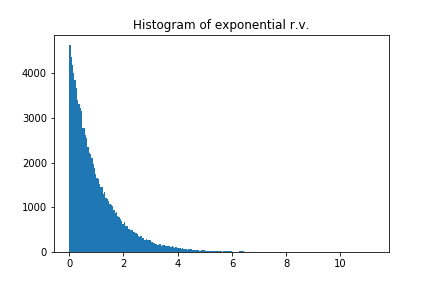
s = expon.rvs(size=obs)

plt.hist(s, bins='auto')
plt.title("Histogram of exponential r.v.")
plt.show()

Now we look at the maxima of the blocks:

blocks = np.empty([n,k])
for i in range(n):
    blocks[i,:] = s[k*i:k*(i+1)]

maxima = np.empty(n)
for i in range(n):
    maxima[i] = np.max(blocks[i,:])

plt.hist(maxima, bins='auto')
plt.title("Histogram of block maxima")
plt.show()

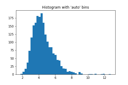
We can see that it looks like a Gumbel distribution as expected. We use scipy’s functions to fit the corresponding curve. We will see in the next entries how can we fit such curves.

from scipy.stats import gumbel_r

params = gumbel_r.fit(maxima)

fig, ax = plt.subplots(1, 1)
x = np.linspace(0,15, 100)

pdf_fitted = gumbel_r.pdf(x , loc = params[0] , scale = params[1] )
ax.plot(x,pdf_fitted,'r-')
ax.hist(maxima,density=True,alpha=.3, bins ='auto')
plt.show()

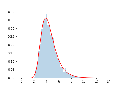
which looks like a very decent fit.

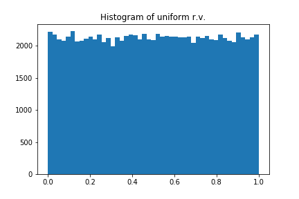
Example 5: consider now uniform random variables $X_i\sim U(0,1)$. We proceed in a similar way as in the previous example: first we sample $X_i$ and take a look at the histogram:

from scipy.stats import uniform

n = 2000
k = 50
obs = n*k

s = uniform.rvs(size=obs)

plt.hist(s, bins='auto')
plt.title("Histogram of uniform r.v.")
plt.show()

Now we construct the blocks and their maxima:

blocks = np.empty([n,k])
for i in range(n):
    blocks[i,:] = s[k*i:k*(i+1)]

maxima = np.empty(n)
for i in range(n):
    maxima[i] = np.max(blocks[i,:])

plt.hist(maxima, bins='auto')
plt.title("Histogram of block maxima")
plt.show()

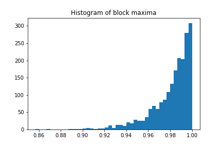
Finally we fit the curve of the Weibull distributioin:

from scipy.stats import weibull_max

params = weibull_max.fit(maxima , floc = 1)

fig, ax = plt.subplots(1, 1)
x = np.linspace(0,15, 100)

pdf_fitted = weibull_min.pdf(x , loc = params[1] , scale = params[2], c = params[0]  )
ax.plot(x,pdf_fitted,'r-')
ax.hist(maxima,density=True,alpha=.3, bins ='auto')
plt.show()

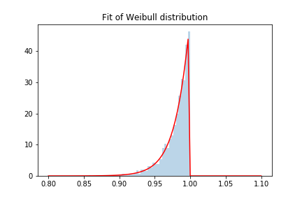
Remark: there are some issues with the Weibull distribution in the scipy library.

Final comments

In this entry we have seen how to find the extremal type of certain distributions by using some tricks. Although, the examples were artficial, and in general these methods do not generalize well, so in the next entry we will see more consistent methods to find the extremal distribution of data using maximum likelihood.