PCA and supervised learning

The situation is this: you have been given data, with several variables $x_1,\dots,x_d$ and a response $y$ that we want to predict using such variables. You perform some basic statistical analysis on your variables, see their averages, ranges, distribution. Then you look at the correlation between these variables, and find that there is some strong correlation between some of them. You decide to perform principal components analysis (PCA) to reduce the dimension of your features to $w_1,\dots,w_m$, with $m < d$. Now you fit your model, and you find that it gives terrible results, even though your PCA variables are capable of explaining most of the variance of the features. What went wrong?

There is a fundamental problem with what we did: PCA is blind to the dependence of the response with respect to the features. In what follows we will explore this situation with a concrete example in low dimension and very simple functions. In higher dimensions the situation can get much worse.

If you like my content, consider following my linkedIn page to stay updated.

How it can go wrong

Suppose that we have data of the form $(x_1,x_2,y)$ where $x_i$ are the features and $y$ is the responde. Suppose that $X_1 \sim \mathcal{N}(0,1)$ and that $X_2 = X_1 + \mathcal{N}(0,0.4)$, that is, $X_2$ is equal to $X_1$ plus some small noise. Essentially, $X_1$ and $X_2$ are the same feature, or in other words, the are highly correlated. Let us generate some data following such distributions:

import numpy as np
np.random.seed(0)

x1 = np.random.normal(0,1,100)
x2 = x_1 + np.random.normal(0,0.4,100)

We can quantify the correlation of these two variables

np.corrcoef(x_1,x_2)

from where we obtain correlation of $0.93$, which is pretty high. Suppose now that our response $y$ is of the form $y = (x_1-x_2) + \mathcal{N}(0,0.2)$, that is, it depends linearly on $(x_1-x_2)$ plus small noise.

y = x1 - x2 + np.random.normal(0,0.2,100)

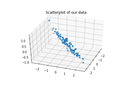
We can plot the triplets $(x_1,x_2,y)$ and see clearly the dependence on $(x_1-x_2)$:

ax = plt.axes(projection='3d')
ax.view_init(elev=40, azim=20)
ax.scatter3D(x1, x2, y)
plt.title("Scatterplot of our data")
plt.show()

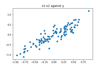
In this setting, a simple linear regression would be able to capture the trend a give good results, as the plot of $(x_1-x_2)$ against $y$ suggests:

plt.scatter(X-Y,Z)
plt.title("x1-x2 against y")
plt.show()

Suppose that we decide to run PCA on our data to reduce the dimensionality. Given that the data is approximately contained in a linear subspace (manifold), it makes sense that we could be able to fit a model using a single feature instead of two. Let us see what happens:

from sklearn.decomposition import PCA

A = np.hstack([x1.reshape(-1,1),x2.reshape(-1,1)])
pca = PCA(n_components=1)
w = pca.fit_transform(A)

Here $w$ is our new feature. We can quantify how much of the variance of our original features $w$ is capable of explaining:

pca.explained_variance_ratio_

We obtain that approximately $96\%$ is explained by $w$, so it seems like a good feature. Suppose now that we try to find a relation between $w$ and $z$. Since the pairs (feature,response) are two dimensional, a simple plot should reveal any relationship between these two feature. Let us see:

plt.scatter(w,y)
plt.title("w against y")
plt.show()

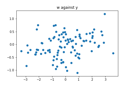
Surprise, no obvious trend! What happened? In order to understand this, we need to think about what PCA is really doing.

A bit about PCA

Let us see with a bit more details what we are doing with PCA: for the features $x_1,x_2$, we construct the covariance matrix $C$ with entries $C_{i,j} = \operatorname{cov}(x_i,x_j)$, then look at the eigenvalue $\lambda_1$ of largest module and its associated eigenvector $u_1$ (which for convenience we take of norm equal to 1), and then project our data onto that vector, that is, we look at the points $w = (x_1,x_2)\cdot u_1$. We will not go into the details why this is what we do to find the directions that maximize the variance, but we will see what happens when we do this in our case. If the vectors $x_1$ and $x_2$ are highly correlated, then the covariance matrix will be very close to the matrix [[1,1],[1,1]] The eigenvalues of this matrix are $\lambda_1=2, \lambda_2=0$, with associated vectors $u_1 = \frac{1}{\sqrt{2}}(1,1)$ and $u_2 = \frac{1}{\sqrt2}(-1,1)$. Thus, we project our data onto the vector $u_1$, obtaining the new feature $w = (x_1,x_2)\cdot u_1 = \frac{1}{\sqrt{2}}(x_1 + x_2)$. We can check that the feature $w$ that we obtained using PCA is essentially $(x_1+x_2)$ by plotting $(x_1+x_2)$ against $y$ and observing the plot is virtually the same as the one we obtained when we plotted $w$ against $y$:

plt.scatter(x1+x2,y)
plt.title('x1+x2 against y')
plt.show()

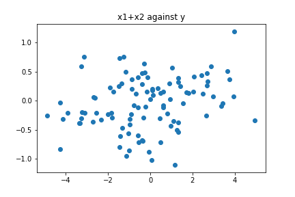
In this sense, while PCA is capable of obtaining the feature that captures most of the variance, it is not aware about how this feature and the response are related. Our final comment: be careful when using PCA in supervised learning, and always perform evaluation before and after applying PCA so we are able to spot situations like the one shown here. Thanks to my friend Alexis Moraga for making me aware of this phenomenon.