Is overfitting… good?

Conventional wisdom in Data Science/Statistical Learning tells us that when we try to fit a model that is able to learn from our data and generalize what it learned to unseen data, we must keep in mind the bias/variance trade-off. This means that as we increase the complexity of our models (let us say, the number of learnable parameters), it is more likely that they will just memorize the data and will not be able to generalize well to unseen data. On the other hand, if we keep the complexity low, our models will not be able to learn too much from our data and will not do well either. We are told to find the sweet spot in the middle. But is this paradigm about to change? In this article we review new developments that suggest that this might be the case.

If you like my content, consider following my linkedIn page to stay updated.

Revising bias and variance

While we framed it as conventional wisdom, the bias/variance trade-off is based on the observation that the loss functions that we minimize when fitting models to our data can be decomposed as

where the error term is due to random fluctuations of our data with respect to the true function which determines responses from features, or in other words, we can think of it as noise on which we do not have control. For the purpose of this entry, we will suppose that the error term can be taken to be zero.

When we fit models to our data, we try to minimize the loss function on the training data, while keeping track of it evaluated on the test data. The bias/variance trade-off means that when we lookt at the test loss as a function of complexity, we try to keep it minimal by balancing both the bias and the variance. This is normally explained with the conventional U-shaped plot of complexity vs loss:

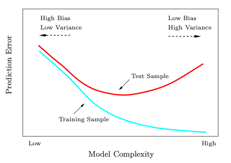
We see that low complexity models do not generalize well, as they are not strong enough to learn the patterns in our data, while high complexity models do not generalize well either, as they learn patterns which are not really representative of the underlying relationship between features and responses. Thus, we look for the middle ground. There have been signs (which can be traced back to Leo Breiman, Reflections after refereeing papers for nips 1995) that this paradigm must be re-thought and that there might be more to it. I am by no means giving an extensive literature review on this, but I will point out some articles which seem particularly interesting in this regard.

Understanding deep learning requires re-thinking generalization

The article Understanding deep learning requires re-thinking generalization by Zhang et al suggested that we should revise our current notions of generalization to unseen data, as they can become meaningless in the examples they exhibit. More concretely, they look at the (empirical) Rademacher complexity, and examine if it is a viable candidate measure to explain the incredible generalization capabilities of the state-of-the-art neural networks

. Suppose that our data has points $\{ (x_k,y_k) : k = 1\dots n\}$ and we are trying to fit functions from a class $\mathcal{H}$, that is, we are trying to find $h\in\mathcal{H}$ such that $h(x_k)$ is as close to $y_k$ as possible, while keeping the error on new samples low. In order to see how flexible for learning the class $\mathcal{H}$ is, consider Bernoulli random variables $\sigma_1,\dots,\sigma_n \sim \operatorname{Ber}(1/2)$ taking values on $\{-1,1 \}$, which we think as a realization of labels for our points $\{x_1,\dots,x_n \}$. A fixed function $h\in\mathcal{H}$ performs well if it outputs the correct label for most points, and since the outputs are $1$ and $-1$ with equal distribution, a good performance would mean that the average

is close to one, as a correct prediction adds one to the sum (both $\sigma_k$ and $h(x_k)$ have the same sign in this case), while an incorrect prediction subtracts one to the sum (the factors have opposite signs). We can find the optimal function in the class by simply taking the supremum over $h$:

The above number quantifies how well the class $\mathcal{H}$ is able to learn a particular realization of labels $\sigma_1,\dots,\sigma_n$. To measure the overall generalizing power of the class $\mathcal{H}$, we look at the average $r(\sigma)$ for all realizations, so we can measure how well the class $\mathcal{H}$ is able to perform over all balanced problems:

We call this number the Rademacher complexity of $\mathcal{H}$. Zhang et al put this measure to a test: they found that multiple modern neural networks architectures are able to easily fit randomized labels. In other words, they took data $\{(x_k,y_k), k = 1,\dots, n \}$ and applied permutations $\phi\in S_n$ to the labels and then trained neural networks on the new data $\{(x_k,y_{\phi(k)}), k = 1,\dots, n \}$, which was capable of achieving near zero train error. These were the same networks that yield state-of-the-art results, so their conclusion is that Rademacher complexity is not a measure capable of explaining the great generalization potential of these networks. In their words:

This situation poses a conceptual challenge to statistical learning theory as traditional measures of model complexity struggle to explain the generalization ability of large artificial neural networks.

They also looked at different measures, such as VC dimension and fat-shattering dimension, for which they have the same conclusions. We are in need then of re-thinking how to measure the complexity of our models.

To understand deep learning we need to understand kernel learning

The follow-up article To understand deep learning we need to understand kernel learning by Belkin et al dives deeper into the phenomenon studied in the previous article, and provides evidence that overfitting models with good generalization results are not a characteristic of deep neural networks, and it is in fact, something we can see in more shallow models. We will not go into further details of this paper, as we just want to remark that the phenomenon is wider than deep learning.

Reconciling modern machine learning practice and the bias-variance trade-off

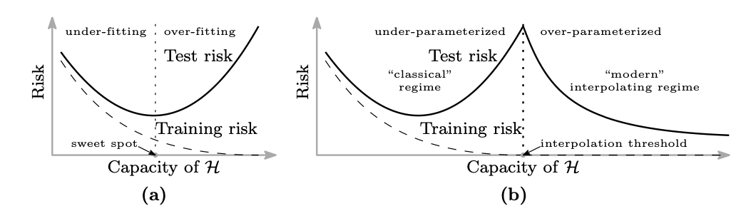
In Reconciling modern machine learning practice and the bias-variance trade-off by Belkin et al, we see again strong signs that the classical bias/variance trade-off picture is incomplete. In their paper, the authors show evidence that (shallow) neural networks and decision trees (and their respective emsembles) exhibit a different behavior to the classical U-shape curve for the test error as a function of the complexity of the model (number of parameters). It is observed that there is threshold point (called interpolation threshold) for which more the training error becomes zero (that is, the model has effectively memorized the data) and the test error is high. Typically this point is presented (if so) at the rightmost of the test error against complexity graph. In the paper, the authors show that beyond the interpolation threshold, the test error starts decreasing again, while the training error stays minimal.

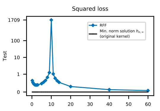
We can see that after the interpolation threshold, the test error decreases again. The x axis represents the numbers of features $\times 10^3$.

The U shape is only the first part of a larger picture.

The authors explain this new regime in terms of regularization: when we reach the interpolation threshold, the solutions are not unique. In order to choose the solution which is optimal in some sense, we can pick the one which gives minimal $\ell^2$ norm to the vector of parameters defining the model. In the case of a shallow neural network, this corresponds to minimizing the norm in the repoducing kernel Hilbert space corresponding to the Gaussian kernel (i.e., an infinite dimensional model). As we expand the class of functions over which we look for our solution, this gives more room to find a candidate with smaller $\ell^2$ norm for the coefficients, acting as a regularization term for the solutions interpolating the data. This mechanism turns out to be an inductive bias, meaning that we strengthen the bias of our already overfitting models.

Benign Overfitting in Linear Regression

The previous paper showed strong evidence for a double descent behavior in the test error against complexity curve: after the interpolation threshold, the test error goes down again. In Benign Overfitting in Linear Regression, Bartlett et al characterize the phenomenon in the setting of linear regression. More precisely, for i.i.d. points $(x_1,y_1),\dots,(x_n,y_n),(x,y)$, we want to find $\theta^*$ such that $\mathbb{E}(x^T\theta^* - y) = \min_{\theta}\mathbb{E}(x^T\theta - y)$. For any $\theta$, the excess risk is

which measures the average quadratic error of our estimations using $\theta$ with respect to the optimal estimations. The article gives upper and lower bounds for the excess risk of the minimum norm estimator $\hat\theta$, defined by

where $X$ is the matrix containing all the realizations $(x_1,\dots,x_n)$ of $x$ as rows and $Y$ is similarly defined for $y$. The bounds in the paper depend of the notion of effective ranks of the covariance matrix of $x$, $\Sigma = \mathbb{E}[xx^T]$, defined by

wheere $\lambda_i$ are the eigenvalues of $\Sigma$ in decreasing order.

Final words

We have seen throughout this article that the notions of complexity need to be re-thought, as well as the traditional idea that bias/variance trade-off is a static picture. There is hard evidence, both theoretical and practical, by means of experiments as well as the daily practices of many ML practitioner, that overfitting is not necessarily a bad thing, as long as we keep control of the test error and observe decay of it after the interpolation threshold. It is worth pointing that for this to happen, it is necessary to have a number of parameters much higher than the number of points in the dataset (taking into account the number of dimensions of each point), which can become computationally expensive. We may see in the future practices like this more often, and maybe one day the books will have to be changed and the bias/variance trade-off will be a thing of the past. In pragmatic terms, as long as it works, we can keep doing it!

Images from: 1 Elements of Statistical learning,

2, 3 Reconciling modern machine learning practice and the bias-variance trade-off

Thanks to Juan Pablo Vigneaux and Bertrand Nortier for pointing my interest to some of the papers discussed here.