Extreme value theory I

In this entry I will discuss some of the introductory concepts of Extreme Value Theory (EVT). This theory is concerned with the asymptotic behavior of the extremes events of a stochastic process, in particular, the distributional characteristics of the maximum order statistics, which will be the focus of this entry. We will first look at i.i.d. processes and then move on to processes with non-trivial dependence. The exposition is based on the book An Introduction to Statistical Modeling of Extreme Values by Stuart Coles. I will also try to use this as a way to showcase the different libraries of python that allow us to work with EVT.

If you like my content, consider following my linkedin page to stay updated.

A degenerate distribution

Let $(\Omega,\mathcal{B},\mathbb{P})$ be a probability space. Consider an i.i.d. process $\{ X_n \}$ with distribution function $F$, that is, $F(s)= \mathbb{P}\{ X_1 \leq s \}$. We are interested in the maximum order statistics: define $M_n:= \max\{X_1,\dots,X_n \}$. We try to find the limiting distribution of $M_n$: let $x\in\mathbb{R}$, then

If $F(x) < 1$ then $(F(x))^n \to 0$ and if $F(x) = 1$ we have $(F(x))^n = 1 \to 1$, hence, the limiting distribution is degenerate. This is no surprise: as we draw more and more samples from our distribution $F$, one of two things is bound to happen:

1. If the support of the distribution $F$ is bounded, we will eventually see peaks $X_{n_k}$ arbitrarily close to the endpoint;
2. If the support of the distribution $F$ is unbounded, then we will see observations $X_{n_k}$ which are arbitrarily large.

This seems to kill the idea of obtaining some asymptotic information of the distribution of $M_n$, but there is a trick that we are well acquinted with: recall that if we consider the sums $S_n:=X_1+\dots + X_n$, then the averages $S_n/n$ converge almost surely to $\mathbb{E}(X_1)$ (Law of large numbers) and the variance of $S_n/n$ is $\mathbb{V}(S_n/n) = \sigma^2/n \to 0$. This implies that the limiting distribution of $S_n/n$ is degenerate too. But recall from the Central limit theorem that if we center and scale $S_n$, we can obtain information about its asymptotic distribution:

In this situation, we proceed to do the same: consider sequences $a_n$ and $b_n$, and we will study the problem

A classification theorem

One of the groundbreaking theorems in EVT is the Fisher-Tippett-Gnedenko theorem, which gives a fundamental insight on the limiting distribution of $M^*_n$:

Theorem (Fisher-Tippett-Gnedenko, Extremal types theorem): suppose that there exist constants ${a_n > 0}$ and ${b_n}$ such that the distribution $G$ of $M^*_n$ is non-degenerate. Then $G$ belongs to one of the three families:

1. $G(z) = \exp \left\{-\exp \left[-\left(\dfrac{z-b}{a}\right)\right]\right\}$, for $z\in\mathbb{R}$,

2. $G(z) = 0 \text{ if } z \leq b$ and $G(z) = \exp \left\{-\left(\frac{z-b}{a}\right)^{-\alpha}\right\} \text{ if } z>b$.

3. $G(z) = \exp \left\{-\left[-\left(\frac{z-b}{a}\right)^{\alpha}\right]\right\} \text{ if } {z<b}$ and $G(z) = 1 \text{ if } z \geq b$,

for parameters $a > 0$, $b\in\mathbb{R}$ and $\alpha >0$. Note: $b$ and $a$ are NOT the mean and variance of the distribution.

The distributions $G$ from conditions 1, 2 and 3 are called Gumbel, Fréchet and Weibull families respectively. Not that the theorem does not ensure the existence of constants $a_n,b_n$ yielding a non-degenerate distribution. There are conditions which allow us to say which family the distribution will converge to, but we postpone such conditions for later. First we note that it is possible to write the three families as part of a single bigger family, the generalized extreme value distribution (GEV):

where $z$ is in the set $\{z: 1+\xi(z-\mu) / \sigma>0\}$ and the paramters are such $\mu \in\mathbb{R}$, $\sigma > 0$ and $\xi\in\mathbb{R}$. Here $\mu$ is called the location parameter, $\sigma$ is the scale parameter and $\xi$ is the shape parameter. The distributions of type 2 and 3 can be obtained setting $\xi > 0$ and $\xi < 0$ respectively, while the distribution of type 1 can be interpreted as the limit case when $\xi \to 0$. The inclusion of all the families into a single larger family is convenient, as for when finding the distribution in concrete cases, we do not need to assume a priori that it will belong to any of the three classes.

Note that the theorem is of a similar flavor to the Central limit theorem: when there is distributional convergence, regardless of the initial distribution $F$, the centered and scaled maximum will have convergence to a GEV distribution.

If $M^*_n$ has asymptotic distribution $G(z)$, then we can see that

can be rewritten as

where $G^*$ is another GEV distribution. Thus, we can think that $M_n$ will also have an approximate GEV distribution.

A look at the distributions

In this section we will have a quick look at the distributions from the GEV family and how to work with them in python. For most of this article we will use the scipy library and its functionalities:

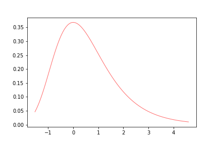
1. Gumbel distribution: consider a type 1 distribution. In general scipy has different conventions for the parameters of the EVT distributions so we will not go into the details of that yet, as we only wish to have a picture in mind of how the distributions look like.

import matplotlib.pyplot as plt
from scipy.stats import gumbel_r

x = np.linspace(gumbel_r.ppf(0.01),gumbel_r.ppf(0.99), 100)
plt.plot(x, gumbel_r.pdf(x),'r-', lw=1, alpha=0.6, label='gumbel_r pdf')
plt.show()

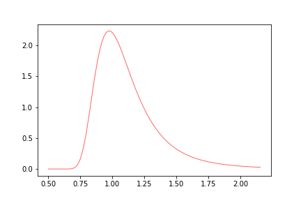
1. Fréchet distribution:

#frechet
from scipy.stats import invweibull

c = 6
x = np.linspace(0.5,invweibull.ppf(0.99, c), 100)
plt.plot(x, invweibull.pdf(x, c),'r-', lw=1, alpha=0.6, label='frechet pdf')
plt.savefig('frechet.png')
plt.show()

1. Weibull distribution:

#weibull
import matplotlib.pyplot as plt
from scipy.stats import weibull_min

c = 1.5
x = np.linspace(weibull_min.ppf(0.01, c),weibull_min.ppf(0.99, c), 100)
plt.plot(x, weibull_min.pdf(x, c),'r-', lw=1, alpha=0.6, label='weibull_min pdf')
plt.savefig('weibull.png')
plt.show()

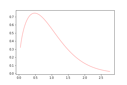
In general if we vary the parameters of the distributions we can observe different qualitative behaviors. We can also see that the distributions are skewed, and present interesting tails behaviors, which we will go through in the following notebooks.

Conclusion

We have seen that the Fisher-Tippett-Gnedenko provides a powerful tool to find the limiting distributions of the extreme values. While it does not provide an algorithm to find exactly which of the three types of distributions we are dealing with. We will see in the next post that the theorem provides enough information so that with a little bit of work, we can find exactly the type of EVT distribution. We will also study methods of estimating the parameters of the corresponding distribution, allowing us to give a first step on EVT inference and predictions.