Confidence intervals

Confidence intervals represent one of the most powerful tools used by statisticians/data scientists. The allow us to quantify the uncertainty of our predictions, which proves crucial when making important decisions. In this entry we will take a first dive into this topic, finding confidence intervals for means of i.i.d. processes.

If you like my content, consider following my linkedin page to stay updated.

The central limit theorem

In previous entries we have seen how the Law of large numbers, the Central limit theorem (CLT) and the principle of Large deviations give a wide description of the asymptotic behavior of averages of i.i.d. They describe the almost sure behavior, the distribution of the fluctuations, and the decay of extreme probabilities. This time, we will use the CLT to study the probability of giving estimates which are close enough to the mean up to a certain confidence level. Recall that if $X_1,X_2,\dots$ is and i.i.d. sequence with finite variance $0<\sigma^2 < \infty$ and mean $\mu$, and denote $S_n := X_1+\dots +X_n$, $\bar X:= S_n/n$. The CLT then can be stated as

where $\mathcal{N}(0,1)$ is the standard normal distribution. If we scale and translate, we obtain the equivalent asymptotics

These results will be useful in the next section.

Estimating the mean

Suppose we are in a situation where we observe i.i.d. data $X_1,X_2,\dots$ with mean $\mu$ and variance $0<\sigma^2<\infty$ (the question of how we know the data is i.i.d. is the topic for a whole another entry!). Suppose that we are interested in estimating the mean $\mu$. For this section, suppose that we know the variance $\sigma^2$ (which in real life is a pretty unlikely situation). A natural candidate to estimate $\mu$ is $\bar X$, which we call the sample mean. We can see from the results following from the CLT that:

• If we compute the sample mean, as we gather more data, it converges in distribution to the true parameter $\mu$, with decreasing variance $\sigma^2/n$. This means that if we perform many random samples of $\bar X$ and plot the corresponding histogram, it will tend to concentrate around $\mu$ and the curve will become more and more narrow.

This provides a good starting point to quantify how certain we are that our estimate $\bar X$ is close enough to $\mu$, as we can actually measure probabilities using the normal distribution $\mathcal{N}$. Denote

which we call the Z statistic. Note now that $|Z| \leq \eta$ if and only if

This means that if we can control the probability that the Z statistic is within a certain interval, we are exactly controlling the probability that the true value of the parameter is within an interval that we can explicitely write down. More concretely, we have that

where $\Phi$ is the cumulative distribution function of the standard normal distribution $\mathcal{N}(0,1).$ For instance, if we wanted an interval $I$ which contains $\mu$ with probability $\alpha = 0.95$, then we need to find $\eta$ such that $2\Phi(\eta) -1 = 0.95$. One can numerically invert $\Phi$ or look its approximate values in a table and see that this means that $\eta \approx 1.96$ (see for instance here: look for the area in the table and find in the axis the correspondig value of $\eta$). This shows where the classical “1.96” number comes from. We call the interval $[\bar X - \eta\frac{\sigma}{\sqrt{n}},\bar X + \eta\frac{\sigma}{\sqrt{n}}]$ a confidence interval for $\mu$ when $\sigma^2$ is known.

We can interpret the previous result as follows: if we draw samples and construct a sequence of confidence intervals $I_1,\dots,I_n$, then the proportion of intervals that contain $\mu$ is given by $\alpha$. In the previous example, $95$ out of $100$ intervals contain $\mu$. We stress that this is an asymptotic result, as it relies both in the law of large numbers and the central limit theorem approximations.

Note that the width of the interval is determined by three factors:

1. The size of the variance of the distribution, ie, $\sigma^2$: if the distribution has high variance, then we are less likely to capture $\mu$, since our data may be skewed away from its mean.
2. The amount of data we have. This one is obvious: the more data, the smaller $\frac{1}{\sqrt n}$, since we know more about our distribution if we sample more data.
3. The confidence level $\eta$: note that $\eta$ is determined by the equation $F(\eta) = (\alpha+1)/2$ and that $F$ is an non-decreasing function (it is a CDF). This means that the closer we want $\alpha$ to be to $1$, the bigger $\eta$ is (assuming that $F$ has no right endpoint).

But we do not know $\sigma^2$

Yes, that is a problem for the method described before. One would be tempted to replace the unknown quantity $\sigma^2$ with the estimator $s^2$ given by

and then estimate $\mathbb{P}(\mu \in I)$ by taking

where we replaced $\sigma$ by $s$. It turns out that the statistic

is not normally distributed, hence we cannot use the same idea as above. Luckily, there is a work around: William Sealy Gosset, aka, Student, proved that under certain assumptions$^*$ the statistic $T$ has a particular distribution, called Student’s t-distribution, and is given by

where $k$ is a parameter called the degrees of freedom, and $\Gamma(\cdot)$ is the gamma function. We can see the graph of the density for different choices of $k$ in the plot below.

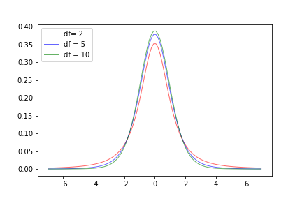
For the $T$ statistic, $k=n-1$. Qualitatively, the t-distribution has a bell shape and is symmetric, so it looks like the Gaussian distribution, but has some different properties. For instance, we can see from its density that it has heavier tails than the normal distribution (it does not decay exponentially). If we call $F_k$ the CDF of the t-distribution, then we can apply the same technique as above to construct confidence intervals when $\sigma^2$ is not known:

The comments on the width of the resulting confidence intervals apply similarly here, so we will not go over them again. What is worth mentioning is that as $n\to\infty$, the t-distribution with $n-1$ degrees of freedom tends to look like the normal distribution. Arguments for this can be found here. There is a big discussion on whether to use the t-distribution for large values of $n$ or not, but we will not go in that direction for now. The only remark we make about it is that for $\alpha = 0.95$ and a large enough number of degrees of freedom, we have that $\eta \approx 1.96$ as well, giving practically the same confidence interval as in the $Z$ statistic case.

$^*:$ The assumptions for this result to hold are the following: if we write the T statistic as $T= \frac{\bar X - \mu}{\sigma/\sqrt{n}} = \frac{Z}{s}$ where

1. $Z$ is has standard normal distribution (ie, $Z\sim \mathcal{N}(0,1)$);
2. $s^2$ has chi-squared distribution with $n-1$ degrees of freedom;
3. $Z$ and $s$ are independent

These assumptions hold in the case when $X_i\sim \mathcal{N}(\mu,\sigma^2)$ (see Cochran’s (see also here) and Basu’s theorem). This is usually how the t-distribution is defined: the ratio of a normal and a chi-squared distribution. Obtaining the density of the t-distribution is a matter of integration and careful analysis of integral kernels (see here and here).

Final comments

We have seen how to construct confidence intervals for the sample mean by using the T-statistic. In future notebooks we will explore confidence intervals for different estimators, as well as their use in hypothesis testing.

References

• Statistical inference, Berger & Casella,
• Statistical data analysis, Cowan