The ergodic theorem

In previous entries (see here and here) we have seen how the weak and the strong law of large numbers gives us asymptotics for the averages of i.i.d. sequences. While the assumption of independence allows us to apply this result in many different contexts, it is still a quite strong assumption. The ergodic theorem constitues a generalization where we allow a certain degree of dependence between the random variables being considered.

If you like my content, consider following my linkedin page to stay updated.

Dynamical systems

In order to formulate the ergodic theorem, we need some background from dynamical systems. Consider a probability space $(X,\mathcal{B},\mu)$, which we call the phase space. If our measure space is of finite measure, we can normalize and turn it into a probability space, while if the space is not of finite measure, most of the results we will talk about do not hold. We also consider a measurable transformation $T\colon X\to X$, which we call the dynamics of the space. We think of $T$ as a deterministic law of evolution of the phase space. In order to observe the phase space, we consider measurable functions $f\colon X\to\mathbb{R}$, which we call observables or potentials. We think of observables as internal characteristics of the space, such as its internal energy. We say that $T$ preserves $\mu$ if

for all $A\in\mathcal{B}$. This property is equivalent to the fact that for any integrable observable $f\in L^1(\mu)$, the time series $Z_n=f\circ T^n$ is identically distributed. We are interested in the averages of $f$ as we compose it with the iterates of $T$:

for generic points $x\in X$.

Example: consider $X=[0,1]$ equipped with the Borel sigma-algebra and the Lebesgue measure $m$ restricted to $X$. Consider also the transformation $T(x) = 2x \pmod 1$. Then $T$ preserves $m$.

Ergodicity

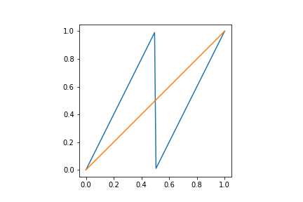
In order to have a law of large numbers in the above context, we need to assume some irreducibility conditions. Consider the dynamics in the picture:

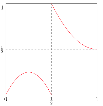
and assume that $T$ preserves the Lebesgue measure. Note that $T([0,1/2])\subset [0,1/2]$. Consider the observable $f (x)= 1_{[0,1/2]}(x)$, where $1_A$ is the indicator function of the set $A$. Suppose we have that the averages of $f\circ T^k$ converge to a constant $c$ almost surely. This would mean that for almost all points $x\in [0,1/2]$, we have that

The left-hand side is the number of iterates $T^k(x)$ are in $[1/2,1]$, divided by $n$. But given $T([0,1/2])\subset [0,1/2]$, the left-hand side is zero for all $x\in [0,1/2]$, hence $c$ must be equal to $0$. Similarly, if we take $f (x)= 1_{[1/2,1]}(x)$, we obtain that $c$ must be equal to $1$.

From the example above we conclude that an irreducibility condition must be necessary in order for a LLN to hold in this context. It turns out that this is not only necessary but sufficient. Let’s formulate precisely the above condition: suppose that if $T^{-1}A = A$ for $A\in\mathcal{B}$, then $\mu(A) = 0$ or $\mu(A) = 1$. We say that $\mu$ is ergodic with respect to $T$.

The ergodic theorem

We have already all the elements to formulate the ergodic theory.

Theorem (Birkhoff): suppose that $T$ preserves the probability measure $\mu$, and that this is ergodic. For any integrable observable $f\in L^1(\mu)$, we have that

for $\mu$-almost every point $x$.

The proof of this result involves a lot of work and we postone it for now. We see now how this generalizes the LLN: let $\{ Z_n\}$ be a sequence of i.i.d. random variables on $(\Omega,\mathbb{P})$. Define $X:=\mathbb{R}^\mathbb{N}$ with the sigma-algebra generated by the cylinders and the dynamics $\sigma\colon X\to X$ given by $\sigma(x_1,x_2,\dots) = (x_2,x_3,\dots)$. We call this map, the left shift on $X$. We can think of each realization of the sequence $\{Z_n\}$ as an element of $X$ given by $(Z_1(\omega),Z_2(\omega),\dots)$. The random variables $Z_n$ define a probability measure $\nu$ on $\mathbb{R}$. Consider the product $\mu=\nu^{\otimes\mathbb{N}}$ on $X$, and the fact that $\{Z_n\}$ are i.i.d., implies that $\sigma$ preserves $\mu$. Finally, consider the observable $f\colon X\to\mathbb{R}$ given by $f(x_1,\dots)=x_1$. Proving that $\mu$ is ergodic requires a bit more work: see here. Applying the ergodic theory to $(X,\mathcal{B},\mu,\sigma,f)$ and noting that $f\circ\sigma^n(\omega) = Z_{n+1}(\omega)$ for $n\geq 0$ gives that

for $\mathbb{P}$ almost every realization as we wanted to prove.

Applications to Markov chains

One of the biggest applications of the ergodic theorem is proving that Markov chains have a LLN. In what follows we will consider only homogeneous Markov chains. Recall a stochastic process $\{Z_n\}$ on $(\Omega,\mathbb{P})$ taking values in a finite/countable set $S$ is called a (discrete time) Markov chain if

for all $z,z_n,\dots, z_1 \in S$ and $n\geq 0$. We call $\mathcal{S}$ the space of states. The Markov chain is characterized by the probabilities $p_{i} = \mathbb{P}(Z_{1} = i)$ and $p_{ij} = \mathbb{P}(Z_{n+1} = j | Z_n = i)$ for all $i,j\in\mathcal{S}$ and $n\geq 1$. We denote the matrix with entries $p_{ij}$ by $P$ and we call it the matrix of transition probabilities, and the vector with entries $p_i$ by $p$, which we call the initial distribution. Before diving into the LLN, we will recall some properties of Markov chains.

The idea behind the model of Markov chains is that we jump from one state $i$ in $\mathcal{S}$ to another state $j$ at random, and the probability for that jump is given by $p_{ij}$. The dynamic properties of this process are interesting, and can be classified in terms of the matrix $P$. For instance, the probability that after $n$ steps the state is $i$ is given by $(p^T P^n)_i$.

An important question about Markov chains is when can two given states be connected with non-zero probability. We say that two a state $j$ is accessible from the state $i$ if there exists a sequence $(i_0 = i, i_1,\dots ,i_{n-1} , i_n = j)$ such that $P_{i_k i_{k+1}} > 0$ for all $k$. We say that $i$ and $j$ are connected if $i$ is accessible from $j$ and vice versa. Note that being connected is an equivalence relation, and partitions the space of states in classes, which we call communication classes. We say that the Markov chain is irreducible if there is only one communication class.

The asymptotic properties we are interested in are recurrence properties. In order to give the proper definition, we need to define a relevant stopping time. For a state $i$, we define its return time $T_i = \inf{ n > 0 : Z_n =i }$. This gives us the first time before the Markov chain returns to the state $i$. With this we can classify the states in two classes:

1. If $\mathbb{P}(T_i < \infty | Z_1 = i) = 1$, we call $i$ recurrent.
2. If $\mathbb{P}(T_i < \infty | Z_1 = i) < 1$, we call $i$ transient.

In other words, paths either return to their initial state with probability $1$, or there is a positive probability that they never return. In the case that they almost surely return, we can further divide the recurrent states in two classes:

1. A state is positive recurrent if $\mathbb{E}(T_i | Z_{1}=i) < \infty$.
2. A state is null recurrent if $\mathbb{E}(T_i | Z_{1}=i) =\infty$.

All states in a given communication class are either recurrent or transient. If a communication class is recurrent, then all of its elements are either null recurrent or positive recurrent. We can describe now the ergodic theory in the setting of Markov chains:

Theorem: let $\{Z_n\}$ be an irreducible Markov chain. Let $V_i(n)$ the number of visits of the chain to the state $i$ in the first $n$ steps. Then

If $\mathbb{E}(T_i| Z_1 = i) = \infty$, we understand $\mathbb{E}(T_i| Z_1 = i)^{-1}=0$.

This is essentially an equidistribution result: the Markov chain spends proportionaly as much time as the inverse of its return time. In other words, the longer it takes it to return, the less time it spends in that state. Null recurrent states take so long to be visited back that the chain spends virtually no time there. This theorem can be extended to functions on the Markov chain. The proof from the ergodic theorem follows a similar line to what we observed above for i.i.d. sequences: we form a space of sequences, construct an invariant ergodic measure and apply the ergodic theorem to indicator functions.

More about Markov chains can be read here.