Understanding bias and variance

In this notebook we will study the concepts of bias and variance and how can we use them to fit models to our datasets. We will base our exposition in both theory and examples.

If you like my content, consider following my linkedin page to stay updated.

Introduction

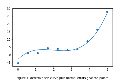
Suppose we have a dataset consisting of $d$-dimensional inputs $x^{(1)},\dots,x^{(m)}$ and real valued outputs/responses $y^{(1)},\dots,y^{(m)}$. We suspect that the responses follow a deterministic rule, but due to factors we cannot measure/control, these deterministic predictions are skewed by a random noise. More precisely, we think there is a function $f:\mathbb{R}^d\to\mathbb{R}$ and random variables $\epsilon^{(k)}:\mathbb{R}^d\to\mathbb{R}$ such that

We are interested in capturing the true deterministic relationship between $x$ and $y$, ie, the function $f$. For this, we propose a model

where $\widehat f:\mathbb{R}^d\to\mathbb{R}$ is a random function depending on the data we have.

Remark: there are multiple possibilities to having the error terms added to the true underlying function. We call this model additive for clear reasons.

Mean squared error

For the problem of how to find the right function $\widehat f$, there are many different approaches. Here we will follow the Mean squared error approach. The central idea of this method is that we will tray to minimize the average of the square of the errors of the predictions made by our predictor function $\widehat f$ with respect to the actual values given by $f$. Since it is not possible for us to know the value of the error, we cannot directly compare $\widehat f$ to $f$ but to $y$. This will induce an irreducible error term. More precisely, we define the mean squared error by

Now, we make some assumptions about the random error in order to have a reasonable theory. We assume that

• The mean of $\epsilon^{(k)}$ is zero.
• The variance of $\epsilon^{(k)}$ is equal to a finite number $\sigma^2$.
• The errors $\epsilon^{(k)},\epsilon^{(j)}$ are independent for $k\neq j$. In other words, all different measurements $y^{(k)}$ are independent.

These two assumptions are very weak: if the mean of $\epsilon$ is not zero, then we can simply substract its mean and add it to the deterministic function $f$, hence $\epsilon-\mathbb{E}(\epsilon)$ is our new error function with zero mean. On the other hand, if the variance of $\epsilon$ was not finite, the we would observe much more sparse data and the situation would be much more delicate. We will assume later on that the errors have a normal distribution $n(0,\sigma^2)$.

Bias and variance

Under the assumptions above, we make the following observations:

• Since $f$ is not random, $\mathbb{E}(f)=f$. This together with the fact that the noise has zero mean, implies that $\mathbb{E}(y)=f$.
• $\text{var}(y) = \mathbb{E}(y^2)-\mathbb{E}(y)^2=\mathbb{E}(f^2+2f\epsilon+\epsilon^2)-f^2= 2f\mathbb{E}(\epsilon)+\mathbb{E}(\epsilon)^2=\sigma^2$.

We define the bias of the model $\widehat f$ by

and the variance by

We can think of the bias as the typical absolute deviation of our predictor $\widehat f$ from the true relation $f$, and the variance as how scattered our predictions will be in average, with respect to its means. Then, we can write the MSE as

Here we remark that $\mathbb{E}(y\widehat f)=\mathbb{E}(y)\mathbb{E}(\widehat f)$ since $\widehat f$ depends on the errors $\epsilon^{k}$ for $k=1\dots m$ and $y$ depends on an error function for a not yet observed point. We conclude that

The last equality has very important consequences:

• The MSE cannot be minimized below the threshold given by the variance of the noise.
• The choice of the model $\widehat f$ can have a substantial influence on how small we can make the MSE.

Unbiased estimators

If we choose $\widehat f$ carefully, we can make $\text{bias} (\widehat f)$ as low as zero. In this case, we say that $\widehat f$ is an unbiased estimator.

Example 1: (sample mean)

Suppose we sample $m$ points $y^{(1)},\dots,y^{(m)}$ coming from a common distribution, and we are interested in estimating the population mean $\mu$. We propose the estimator

We can compute now its bias:

since all the points $y^{(k)}$ have the same mean. Thus, $\widehat\mu$ is an unbiased estimator.

Example 2: (sample variance, uncorrected)

Suppose now that from the same sample as in the previous example, we want to estimate now their variance. We propose the estimator

for $\sigma^2$. A similar (but much more tedious) computation can show that

and hence

where $\sigma^2$ is the variance of the distribution yielding the data $y^{(k)}$.

Example 3: (sample variance, corrected)

If we take the estimator

then $s^2$ is an unbiased estimator of $\sigma^2$: $\mathbb{E}(s^2)=\sigma^2$. This correction is known as Bessel’s correction.

Minimizing the variance

Just as for the bias, if we choose our estimators carefully, we can control their variance and hopefully minimize the MSE.

Example 4: (variance of the sample mean)

In the setting of example 1, we want to compute $\text{var} (\widehat\mu)$.

We can see that the variance of the estimator decreases as we gather more data.

Example 5: (variance of the sample variance)

From the previous examples, we have two different estimators $s^2,\overline s^2$ for the variance $\sigma^2$. We have seen that $\mathbb{E}(s^2)=\sigma^2$ and $\mathbb{E}(\overline s^2)=(1-1/n)\sigma^2$. Now if we assume that our samples have normal distribution $n(\mu,\sigma^2)$, it is possible to show that

and

For more general distributions it is possible to compute the variance as well, but the expressions are more involved (see previous link). Observe now that

so the biased estimator $\overline s^2$ has a smaller variance than the unbiased estimator $s^2$.

Bias vs variance tradeoff

We have explored in the previous sections different choices for estimators and how this changes the bias and the variance. At first glance it looks clear that we should take unbiased estimators so the bias contribution to the MSE is zero. Now we will see how this choice is not trivial.

Example 6: (sample variance tradeoff)

From the previous examples we have seen that for a normally distributed population ($n(0,\sigma^2)$), the variance $\sigma^2$ can be estimated with $s^2$ and $\overline s^2$. We have computed the bias and variance of these estimators, and hence we can write the MSE (omitting the noise term which is equal for both of them) as

Observe now that $MSE(\overline s^2)< MSE(s^2)$, thus, the estimator with higher bias ended up having a smaller MSE.

Final remarks

It is important to remark that this situation is more common than one would expect. If we take for example the unbiased estimator $s^2$ for $\sigma^2$, then we may argue that gathering more data we would decrease the MSE, but that is not the situation that we will be in most of the times. Oftentimes we have a fixed dataset and we are trying to find the best estimator for the quantities we want to predict. This implies that from all the available estimators, we need to choose the ones that minimize the MSE by taking into account both bias and variance. This leads to situations such as the one of the examples, where increasing the bias leads to a smaller variance and an overall smaller MSE. In general, more complex models (that have more degrees of freedom) have less bias but have a bigger variance, while simpler models tend to be more biased but have a smaller variance. We will study some examples in depth, particularly, models concerning regression. We will also explore different ways to measure the error, other than MSE, and how they can yield different optimal estimators.

Edit: thanks to Ignacio Alvizu for poiting out the mistake in the last paragraph.