Statistical laws in Dynamical Systems

In this entry I will attempt to introduce some of the fundamental concepts in my research. In particular, I want to discuss the topic of Limit laws in dynamical systems, and the endgoal is to explain our latests results together with Matthew Nicol (University of Houston), Large deviations and central limit theorems for sequential and random systems of intermittent maps. This is a huge topic, and as such I will divide the exposition in multiple articles. In this particular one, I will focus in Central limit theorems and Large deviations estimates for one dimensional maps of the unit interval. The exposition will use the formal notation of probability theory, but the ideas do not require a deep knowledge of the formalism behind probability theory. The code for all the graphics and functions can be found here.

The i.i.d. case

Let $(\Omega,\mathcal{B},\mathbb{P})$ be a probability space. Suppose that ${X_n}$ is an iid process with mean $\mathbb{E}(X_1) = \mu < \infty$ and variance $0 < \mathbb{E}(X_1^2)-(\mathbb{E}(X_1))^2 = \sigma^2 < \infty$. It is a well know that ${ X_n}$ satisfies the following statistical asymptotic laws:

• Law of large numbers: with probability 1, the averages of the process converge to the mean $\mu$: \(\dfrac{S_n}{n}\to \mu \ \mathbb{P}\text{-almost surely},\) where $S_n:= X_1 + \dots + X_n$.

• Central limit theorem: the fluctuations of the sums $S_n$ around the mean are of order $\sqrt{\sigma^2n}$ asymptotically normally distributed: \(\dfrac{S_n - n\mu}{\sqrt{\sigma^2 n}} \Rightarrow \mathcal{N}(0,1).\)

• Large deviations: the probability that the averages are $\epsilon$ away from the mean decays exponentially: \(\mathbb{P}\left\{\left|\frac{S_n}{n} - \mu\right|>\epsilon\right\} \sim \exp(-nc)\) where $c > 0$ is a constant.

These results give a rather complete picture of the asymptotic behavior of the averages of the process, and find a wide variety of applications.

Hyperbolic dynamics: doubling map

The processes considered in the previous section have a property which is rather strong: independence. This means that the outcome of $X_{n+1}$ is independent of the outcome of $X_1,\dots,X_n$ for all $n$, which for applications is often an assumption which does not hold. There are multiple generalizations of the results from the previous section, namely, Markov chains, martingales, etc, but here we will focus in the generalization given by dynamical systems. Instead of working with a completely general theory, we will focus in a particular example: the doubling map. This example has the property of being very easy to handle, but also captures most of the ideas that are present in the general theory. We proceed to introduce the doubling map:

Let $T\colon [0,1]\to [0,1]$ be the map given by $T(x) = 2x \pmod 1$, that is, $T(x) = 2x$ for $x \in [0,1/2)$ and $T(x) = 2x -1$ for $x\in [1/2,1]$.

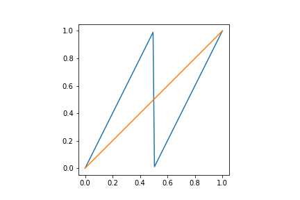
Figure 1: in blue, the doubling map. In orange, the identity map.

The iterates of the map $T$ are of our interest, that is, the compositions of $T^k$.

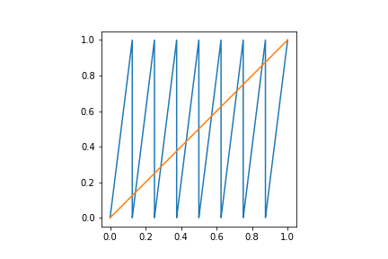
Figure 2: in blue, the third iterate of the doubling map. In orange, the identity map.

The condition of uniform hyperbolicity here can be stated in simple terms: the derivative of the map is strictly bigger than 1 everywhere. How can we construct a stochastic process using a dynamical system? We can think of $[0,1]$ as our sample space, using the Borel sigma-algebra of measurable sets and the Lebesgue measure $m$ as the probability measure. We will consider integrable functions $f\colon [0,1] \to \mathbb{R}$ as our starting random variable (which we call observable), and we will form a sequence of random variables by setting $X_n := f\circ T^n$ for $n\geq 1$. If this sounds complicated, all that it means is that we will sample numbers in $[0,1]$ and observe them through the action of $f\circ T^n$. Note that $m(T^{-1}(A)) = m(A)$ for all $A\in\mathcal{B}$. This implies that all $X_n$ have the same distribution. It is important to note that in general, $X_n$ is not independent of $X_m$ for generic choices of $f$. This means that the results for i.i.d. processes do not directly apply in this setting. Fortunately, there are ways to make these results work

• The ergodic theorem: let $S_n = X_0 + \dots + X_{n-1}$ (Birkhoff sums), then \(\dfrac{S_n}{n} = \dfrac{1}{n}\sum_{k=0}^{n-1}f\circ T^k\to \int f dm \qquad m\text{-almost everywhere.}\)

This result is a direct generalization of the law of large numbers, and holds in great generality. It essentially says that if we average the value of $f$ along the orbit under $T$ of a generic point $x$, then we obtain the spatial average over the whole space. This result can also be interpreted as an equidistribution result: the orbits of generic points tend to spend equal amounts of time in regions of equal size (measure).

The next two results are more delicate, so we will treat them separately from the previous result. We will approach the problem from a numeric perspective.

• Central limit theorem: for this, we start by implementing the dynamics $T$. As we want to iterate the map, we also implement its iterations. The method we use is recursive, which is by no means the most efficient, but more intuitive and simple. We will assume for the sake of simplicity that the input x is always in $[0,1]$.

  def doubling(x,n):
    if n == 0:
        return x
    elif n == 1:
        return 2*x*(x <= 1/2) + (2*x - 1)*(x >= 1/2)
    else:
        return doubling(doubling(x,n-1),1)
  

  We also implement a function that returns the $n$-th sum $S_n = \frac{1}{n}\sum_{k=0}^{n-1}f\circ T^k$. Here again the implementation is not efficient, as we will compute the compositions $f\circ T^k$ more times than we actually need.

  def birkh(x,f,n):
    S = 0
    for i in range(n):
        S += f(doubling(x,i))
    return S
  

  The observable we will consider is an arbitrary choice for reasons that will be explained later. Let $f\colon[0,1]\to \mathbb{R}$ be given by $f(x) = (3x\sin(10\pi x) + 4)/(4 - 3/(10\pi))$.

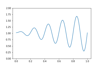
Figure 3: a particular choice of a smooth observable.

The normalization is so that $\mathbb{E}(f)= \int f dm = 1$. It can also be seen that the variance of $f$ is given by $\sigma^2 = (15(-3 + 40\pi^2))/(4(3 - 40\pi)^2)$. We will now simulate a Central limit theorem situation: we construct a random sample from $[0,1]$, evaluate the centered sums $\frac{S_n - n\mu}{\sqrt{n\sigma^2}}$ and construct a histogram to study their distribution. We will also fit a normal curve and find its mean and variance:

def rho(x):
    return (3*x*np.sin(10*np.pi*x) + 4)/(4 - 3/(10*np.pi))

var_rho = (15*(-3 + 40*np.pi**2))/(4*(3 - 40*np.pi)**2)
sample_size = 1000
num_iter = 50

sample = np.random.uniform(0,1,sample_size)
B = (birkh(sample,rho,num_iter) - num_iter)/(np.sqrt(n*var_rho))
plt.hist(B, bins=30, density=True, alpha=0.6, color='g')

mu, std = norm.fit(B)
xmin, xmax = plt.xlim()
x = np.linspace(xmin, xmax, 100)
p = norm.pdf(x, mu, std)
plt.plot(x, p, 'k', linewidth=2)

plt.ylabel('Histogram of fluctuations sums')
title = "CLT: Fit results: mu = %.2f,  std = %.2f" % (mu, std)
plt.title(title)
plt.show()

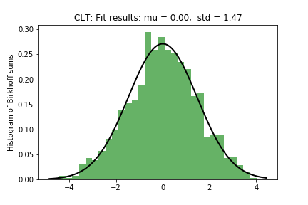
Figure 4: histogram of fluctuations demonstrating their normal distribution.

We can observe that the distribution of the fluctuations is normal, and its parameters are $\hat{\mu}=0$ and $\hat{\sigma^2}=1.4$. This distributional result can be proven using spectral theory, noting that the usual proof of the CLT can be extended to this case by using an argument of Nagaev and Guivarc’h (see Limit theorems in dynamical systems using the spectral method by Sébastien Gouëzel).

• Large deviations estimates: we proceed now to investigate large deviation rates for our observable $f$. For this, we first will look at the distribution of the averages minus the mean, and see, for a fixed threshold $\epsilon > 0$, what proportion of the histogram is beyond the threshold. We are interested in studying how does that proportion change as we make the number of iterations being considered larger. Let us then plot such histograms for different values of $n$ and $\epsilon = 0.1$:

  sample = np.random.uniform(0,1,1000)
  B = np.abs(birkh(sample,rho,n)/n - 1)
  B_close = B[B > epsilon]
  B_away = B[B <= epsilon]
  plt.hist(B_away, bins=30,   alpha=0.6, color='b')
  plt.hist(B_close, bins=30,   alpha=0.6, color='g')
  plt.title('n = %d' % n)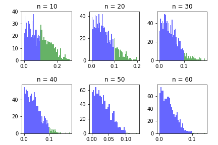
  

  

Figure 5: histogram of the deviations of the Birkhoff sums.

We can see from the figure that the large deviations probability decays as $n$ becomes larger. We will plot such probability for different choices of $n$, for the same value of $\epsilon$:

n = 25
LD = []
epsilon = 0.1
sample_size = 2000

for i in range(1,n):
    sample = np.random.uniform(0,1,sample_size)
    B = np.abs(birkh(sample,rho,i)/i - 1) - epsilon
    LD.append((np.sum(B > 0))/len(B))

plt.plot(LD)
plt.ylabel('Large deviations probability')
title = "Decay of LD probabilities"
plt.title(title)
plt.show()

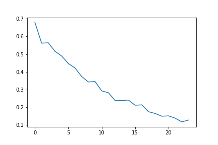
Figure 6: decay of deviations probability.

We can see that the probability decays quite fast. We suspect that in fact it decays exponentially. To check this, we plot the logarithm of the probabilities and fit a curve of degree 1:

z = np.polyfit(range(0,n-1), np.log(L), 1)
p = np.poly1d(z)
plt.plot(p(range(n)))

plt.plot(np.log(L))
plt.ylabel('Log of LD prob')
title = "Linear fit of log of probabilities"
plt.title(title)
plt.show()

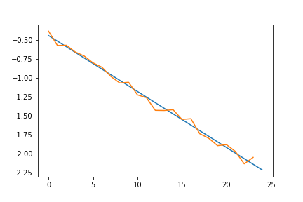
Figure 7: decay of logarithm of deviations probability.

The graph shows that it is a reasonable assumption that the probabilities decay exponentially fast. In fact, this follows from Large deviations in dynamical systems and stochastic processes by Kifer, who built a framework for Large deviations on uniformly hyperbolic maps. The methods he used differ from the methods used in probability theory, as he makes use of the Thermodynamic Formalism, developed, among others, by Bowen, Ruelle, Sinai, Walters.

The role of hyperbolicity

We have mentioned how the hyperbolicity of the doubling map plays a big role in the proofs of statistical laws. The key idea comes from spectral theory. For an essentially bounded observable $f$, we define the composition or Koopman operator $U\colon L^\infty \to L^\infty$ by $Uf = f \circ T$. This operator is interesting by itself, as it allows us to characterize certain dynamical properties in terms of its spectral properties. Rather than working with $U$, we will work with its dual: define $P\colon L^1 \to L^1$ by the relation \(\int f Ug dm = \int Pf g dm\) for all $f \in L^1$ and $g\in L^\infty$. It can be proven that this defines $Pf$ up to a zero measure set. We will refer to $P$ as the transfer operator. One of the fundamental properties of $P$, is that it describes the evolution of densities of measures under the action of $T$: suppose that $\mu$ is a measure which is absolutely continuous with respect to $m$. Then there exists a non-negative function $h\in L^1$ with $\int h dm = 1$ such that $d\mu = h dm$. We can let $\mu$ evolve by considering the pushforward measure $T_*(\mu)(A) = \mu(T^{-1}(A))$ and its iterates. It can be proven that the measure $T_*(\mu)$ is also absolutely continuous with respect to $m$, and its density is $Ph$. The hyperbolicity condition, together with the fact that both branches of $T$ are bijections from their domain to the unit interval, imply that $P$ pushes mass away, in every direction. This has a smoothing effect over densities, as we can see in the next graphic:

def transf(n,x,f):
    S = 0
    for i in range(2**n):
        S += (2**(-n))*f((x+i)/(2**n))
    return S

#This section plots the first iteration of $P$ on $f$
plt.plot(x, transf(0,x,rho))
plt.plot(x, np.ones(len(x)))
plt.xlim([0,1])
plt.ylim([0,2])
plt.grid(True)

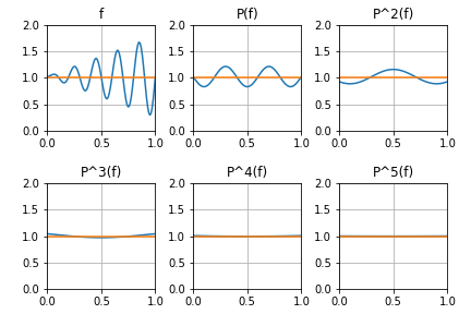
Figure 8: the smoothing action of $P$ on $f$.

When we let $P$ act on a space of sufficiently smooth functions (Lipschitz), it admits a decomposition in two operators: $P = N + \lambda Q$, where $Q$ is a projection and $\dim(\mathrm{im}(P)) = 1$, $N$ is a bounded operator with $\rho(N) < \lambda$ ($\rho(N)$ is the spectral radius of $N$) and $QN = NQ = 0$. This decomposition implies that the spectrum of $P$ consists of $\{\lambda \} \cup \{ |z| < \alpha \lambda \}$ where $\alpha \in (0,1)$. The eigenfunction associated to $\lambda$ is constant, and $\lambda$ is related to the hyperbolicity of $T$. The connection with the usual proof of the CLT comes from the fact that the characteristic function of $S_n$ is nothing but $\int P^n(e^{itS_n}1)dm$, where $1$ is the function constant equal to $1$. Applying perturbation theory (Kato), one can mimic the proof and obtain the corresponding result. It is worth noting that the decomposition $P = N + Q$ does not hold when we do not have uniform hyperbolicity. and that will be the topic of our next entry.

Final words

In this article we have seen how different statistical laws arise when considering the asymptotic behavior of the Birkhoff sums of observables in hyperbolic dynamical systems. In the next entries, I will discuss some results for non-uniformly hyperbolic systems, and what are the main difficulties compared to the case we reviewed in this entry.