Statistical properties in hyperbolic dynamics, part 4

This is the fourth and last post of a series of 4 posts based on the lectures at the Houston Summer School on Dynamical Systems 2019 on Statistical properties in hyperbolic dynamics, given by Matthew Nicol, Andrew Török and William Ott. These notes are heavily edited with added comments, examples and explanations. Any mistake is of my responsibility. Some of the notation has been changed for consistency.

Lecture 4

In the previous three lectures we introduced several methods for studying statistical properties of dynamical systems, such as martingale approximation or quasi-compactness. In this lecture, we are interested in the case of non-autonomous (non-stationary) dynamical systems. We will limit our discussion to the discrete time case. A motivation to consider this kind of systems is to model dynamics which evolve in time, or that we have no certainty of being stationary. This includes systems such as billiards with moving scatterers (heavy particles dynamics), or open systems such systems of genes producing proteins which signal processes that influence back the genes.

Suppose we have a family of dynamics $\{ f_i\}_{i\in\Omega}$ on the same probability space $(X,m)$. In general the transformations $f_i$ will not preserve the measure $m$ and will not exist any measure which is invariant for all transformations. We will assume that the transformations are non-singular with respect to $m$.

In the previous posts, we defined the correlation function for a single transformation: let $T\colon X\to X$ be a non-singular transformation of the probability space $(X,m)$. For observables $\phi,\psi\colon X\to\mathbb{R}$, define their correlation function by

Our first goal is to define a notion analogue to the one of decay of correlations for our non-autonomous setting. In the autonomous case, it is possible to prove a stronger property than decay of correlations: for every pair of observables $\phi,\psi$ with equal expectation,

as $n\to\infty$. Note that this implies decay of correlations. In particular, if $h$ is the density of an invariant measure, then we have that

for all densities $\phi$. This implies that all densities evolve towards the fixed point of $P$.

Let $f$ be the density of an exponential random variable on $[0,1]$, that is

for $x\in[0,1]$, and $g$ the density of a beta distribution with parameters $\alpha = 2$ and $\beta = 10$. Then the evolution of these densities under the action transfer operator associated to the doubling map are shown in the pictures, where $f$ and $g$ are plotted as blue lines, while the uniform distribution is plotted as orange lines:

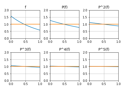
Figure 1: Evolution of exponential distribution

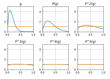
Figure 2: Evolution of beta distribution

We can see that the densities evolve towards the uniform distribution, corresponding to the density of the invariant measure for the doubling map (Lebesgue measure). In particular any two densities get arbitrarily close. This notion is what we will understand as loss of memory in the context of non-autonomous dynamical systems.

To describe the evolution of densities under the action of a non-autonomous dynamics, we need to introduce the dual operator for this system. For every transformation $f_i$, we define call its transfer operator $P_i$. Fix an infinite word $\omega = (\omega_{1},\dots) \in \Omega^\mathbb{N}$, and consider the sequence of compositions $F^n = f_{\omega_n}\circ \dots\circ f_{\omega_1}$. The transfer operator associated to $F^n$ is denoted $P^n$. It is easy to prove that $P^n = P_{\omega_n}\circ\dots\circ P_{\omega_1}$.

We say that the non-autonomous system $\{ f_i\}$ has statistical loss of memory if for every two densities $\rho$, $\zeta$, one has

In the rest of the article we will follow the paper Memory loss for time-dependent dynamical systems by Ott, Stenlund and Young, where they introduced techniques from probability theory in the context of dynamical systems to study the loss of memory of non-autonomous dynamical systems. In particular, they used the method of coupling.

Expanding maps

Consider a compact, connected Riemannian manifold without boundary $M$. A smooth map $f\colon M\to M$ is said to be expanding if there exists $\lambda > 1$ such that

for every $x\in M$ and every vector $v\in T_x M$. We denote by $m$ the Riemannian metric on $M$. The transfer operator $P$ of $f$ can be be explicitely written as

We need to assume some regularity for the maps we are going to sequentially compose. For $\lambda > 1$ and $\Gamma\geq 0$, define

This is the set where we will take the maps from to compose them. We also need to assume some regularity for the densities of the measures we are going to consider. Define

In this setting, we have the following result:

Theorem: for $\Gamma > 0$ and $\lambda > 1$, there exists a constant $\Lambda(\lambda,\Gamma)$ such that for any sequence $\{ f_i \}\in \mathcal{E}(\lambda, \Gamma)$ and any $\phi,\psi\in \mathcal{D}$, there exists $C_{(\phi,\psi)}$ such that

for all $n\geq 0$.

Some ideas of the proof:

First, we look at a scale small enough in the manifold so that we see expansion at the level of the metric in the manifold: fix $\epsilon > 0$ so that $d(f(x),f(y))\geq \lambda d(x,y)$ for all $x,y$ with $d(x,y) < \epsilon$. The next step is to stratify the set $\mathcal{D}$; define $\mathcal{D}_L$ by

Then one has

The next proposition is one the key ingredients of the argument:

Proposition: there exists $L^{*}$ such that for any $L > 0$, there exists $\tau(L) \in\mathbb{N}$ such that for all $\phi \in \mathcal{D}_L$ and $f_i\in\mathcal{E}$, one has $P^n(\phi)\in \mathcal{D}_{L^*}$ for all $n\geq \tau(L)$.

The content of this proposition is that there is a strata of $\mathcal{D}$ which acts as an attracting element under the action of the transfer operator, and once we land in it, we do not leave if if we keep iterating the transfer operator. Note that for $\phi\in \mathcal{D}_{L^*}$ one has $\phi\geq\kappa$ for some $\kappa > 0$. With this in mind, we can study the push-forward measures obtained by composing with the dynamics. If $\phi$ is the density of the measure $\phi dm$, then the density of $(F^n)_{*}(\phi dm)$ is precisely $P^n(\phi)$. The previous observation together with the previous lemma imply that for the densities of the push-forward measure, $P^n(\phi)$, one also has a lower bound by $\kappa$. This means that for two different densities $\phi,\psi \in\mathcal{D}_L$, the push-forwarded densities also share the lower bound $\geq \kappa$. For technical reasons, we think of just $\frac{1}{2}\kappa$ being matched for the two densities $\phi,\psi$. We renormalize the rest of the densities by taking

The next lemma ensures that when we renormalize, we do not lose that much regularity, or in terms of the stratification, we do not do very far from the lower strata on the stratification of $\mathcal{D}$:

Lemma: if $\phi \in \mathcal{D}_{L^*}$, then $\hat{\phi}\in\mathcal{D}_{2L^*}$.

The rest of the proof is just an inductive construction, where we alternate between applying the transfer operator and renormalizing. As doing this keeps increasing the fraction of matched parts for the two densities, the $L^1$ norm of the difference will decrease exponentially. $\square$